Tutorial
This tutorial will guide you through all the steps needed to (i)
load a raw dataset, (ii) preprocess this raw dataset and (iii)
apply the biclustering algorithms supported by BiMS.
In this tutorial we will use the Wine dataset (available in the downloads section), which contains 70 samples labeled in 14 different classes (A-N). At the same time, for each sample there
are 5 replications (i.e. 5 raw spectra).
Contents
1 Load raw datasets
BiMS support data loading from mzML and mzXML raw data formats.
Press the operation File / Load Classified / Raw Data ...
in order to load the wine dataset. A dialog will appear:
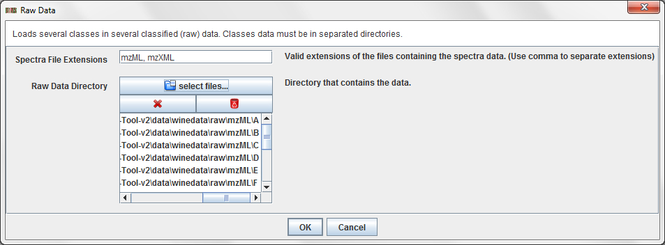
In this dialog, you have to add the folders of the classes which you want to load. Once
you have added all the folders, press OK to load the data.
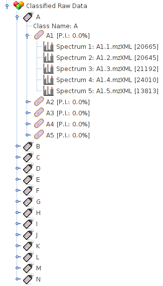
While the spectra are loaded a dialog will inform you of the
progress. After they are loaded, they are added to the
data tree as child of their correspondent Classified Raw Data.
2 Preprocess data
2.1 Preprocess
BiMS allows the users to preprocess raw MS datasets using MALDIquant (for intensity transformation, smoothing, baseline correcion, peak detection and peak alignment) and MassSpecWavelet (for peak detection).
Press the operation Preprocess / Classified Data / Preprocess Classified Data ...
in order to preprocess the wine dataset. A dialog will appear:
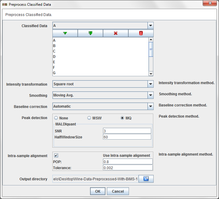
This dialog allows you to choose:
- Classified Data: The Classified Raw Data items from the data tree that you want to preprocess.
- Intensity transformation method: intensity transformation method to use (log, log 10, square root or none).
- Smoothing method: smoothing method to use (moving average or none).
- Baseline correction method: baseline correction method to use (median, convex hull, SNIP, automatic or none).
- Peak detection method: peak detection method to use (MALDIquant, MassSpecWavelet or none).
- Intra-sample alignment: specify wheter intra-sample peak alignment using MALDIquant must be applied. Applying intra-sample alignment means: (i) use MALDIquant to align all the replicates of a sample, then (ii) the replicates are reduced to a single (sample) spectra which contains the peaks that are present in at least POP% spectra.
- Output directory: a directory to store the preprocessed dataset.
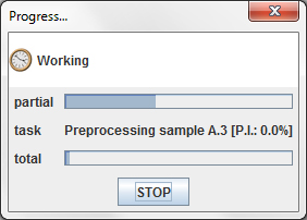
This operation may take a few minuts, depending on your system capacities. While the spectra are preprocessd a dialog will inform you of the progress. After they are preprocessed are ready, they are added to the data tree as child of their correspondent Classified Preprocessed Data.
2.2 Global Alignment
Once each sample has been preprocessed, all the samples in the dataset must be aligned in order to apply the biclustering algorithms.
Press the operation Preprocess / Classified Data / MALDIquant Inter-Sample alignment ...
in order to align the data. A dialog will appear:
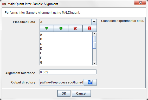
This dialog allows you to choose:
- Classified Data: The Classified Raw Data items from the data tree that you want to preprocess.
- Intra-sample alignment tolerance: alignment tolerance value for MALDIquant.
- Output directory: a directory to store the aligned dataset.
While the spectra are aligned a dialog will inform you of the progress. After the alignments are ready, they are added to the data tree as child of their correspondent Classified Aligned Data.
3 Apply biclustering
BiMS allows the user to apply Bimax and BiBit biclustering algorithms. Press the operation
Analysis / Classified Data / Biclustering Analysis ...
in order to apply biclustering to the preprocessed and aligned wine dataset. A dialog will
appear:
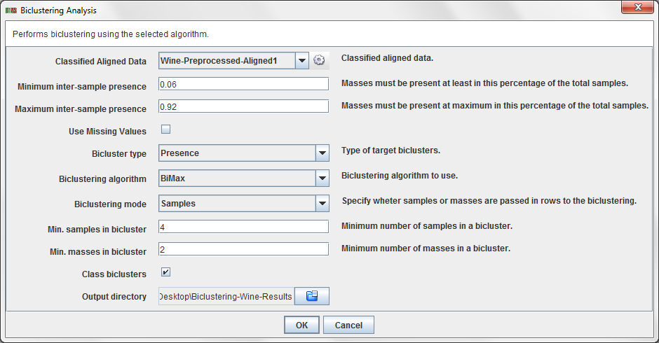
This dialog allows you to choose:
- Minimum inter-sample presence: value betweeen 0 (default) and 1 which specify the minimum percentage of samples where a peak must be present in order to be considered by the biclustering algorithm.
- Maximum inter-sample presence: value betweeen 0 and 1 (default) which specify the maximum percentage of samples where a peak must be present in order to be considered by the biclustering algorithm.
- Use missing values: determine wheter using missing values (NaN) or set them as 0 (default).
- Bicluster type: set if you want to find presence biclusters (that is, biclusters of 1's), absence biclusters (that is, biclusters of 0's) or presence-absence biclusters (that is, biclusters with patterns of 1's and 0's).
- Biclustering algorithm: select the biclustering algorithm to use.
- Biclustering mode: determine if rows of the biclustering input data matrix are samples (default) or peaks.
- Min. samples in a bicluster: minumum number of samples that must be present in extracted biclusters.
- Min. masses in a bicluster:minumum number of peaks that must be present in extracted biclusters.
- Class biclusters:determine wheter the results must be filtered in order to retrieve class-biclusters (biclusters where all the samples are from the same class).
- Output directory: a directory to store the biclustering files.
In this tutorial, we propose you to use the values showed in the previous dialog figure.
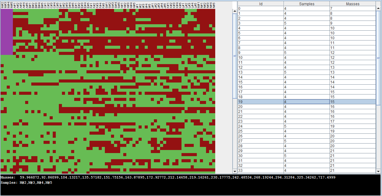
While the dataset is exported and the biclustering algorithm is executed a dialog will inform you of the progress. After the biclustering is ready, it is added to the data tree as child of their correspondent Biclustering.

Finally, the result can be explored with the Biclustering viewer, which is opened by clicking on the biclustering result.